Add Shading to Various Summary Plots

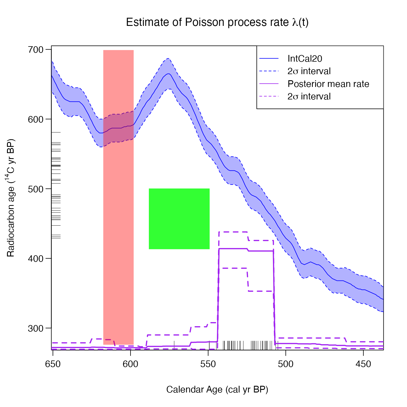
Having plotted the output of the various modelling approaches, add a shaded interval or box to the plot. This function/annotation can be applied after having called any of PlotPosteriorMeanRate, PlotPosteriorChangePoints, CalibrateSingleDetermination, PlotPredictiveCalendarAgeDensity, PlotCalendarAgeDensityIndividualSample, or PlotRateIndividualRealisation.

Usage

AddShadingPlot(
  output_plot,
  x_start,
  x_end,
  y_start = NULL,
  y_end = NULL,
  col,
  alpha = 0.4
)

Arguments

output_plot

The plot onto which you wish to add text

x_start, x_end

The values on the x-axis (calendar age) at which you want the shading to start and end

y_start, y_end

NULL if you want the shading to cover the entire y-axis range. Otherwise (if you want to plot a box) the y-axis values where you want the sahding to start and end

col

The color to be used

alpha

The level of transparency for the shading (0 < alpha < 1) to see the plot underneath. 0 means fully transparent and 1 means fully opaque.

Value

None

Examples

# NOTE: This example is shown with a small n_iter and n_posterior_samples
# to speed up execution.
# Try n_iter and n_posterior_samples as the function defaults.

pp_output <- PPcalibrate(
    pp_uniform_phase$c14_age,
    pp_uniform_phase$c14_sig,
    intcal20,
    n_iter = 1000,
    show_progress = FALSE)

# Default plot with 2 sigma interval
posterior_mean_plot <- PlotPosteriorMeanRate(
    pp_output,
    n_posterior_samples = 100)

# Add transparent red shaded period to plot
AddShadingPlot(posterior_mean_plot,
    x_start = 620, x_end = 600,
    col = "red")

# Add green (more opaque) shaded box to plot
AddShadingPlot(posterior_mean_plot,
    x_start = 590, x_end = 550,
    y_start = 500, y_end = 410,
    col = "green", alpha = 0.8)