Plot Posterior Calendar Age Estimate for an Individual Determination after Joint Calibration

Once a joint calibration function (any of PolyaUrnBivarDirichlet, WalkerBivarDirichlet or PPcalibrate) has been run to calibrate a set of related radiocarbon determinations, this function plots the posterior calendar age estimate for a given single determination. Shown are a (direct) histogram of the posterior calendar ages generated by the MCMC chain and also a (smoothed) kernel density estimate obtained using a Gaussian kernel. The highest posterior density (HPD) interval is also shown for the interval width specified (default 2\(\sigma\)).

For more information read the vignettes:
vignette("Non-parametric-summed-density", package = "carbondate")
vignette("Poisson-process-modelling", package = "carbondate")

Note: The output of this function will provide different results from independent calibration of the determination. By jointly, and simultaneously, calibrating all the related \({}^{14}\)C determinations using the library functions we are able to share the available calendar information between the samples. This should result in improved individual calibration.

Usage

PlotCalendarAgeDensityIndividualSample(
  ident,
  output_data,
  calibration_curve = NULL,
  plot_14C_age = TRUE,
  plot_cal_age_scale = "BP",
  hist_resolution = 5,
  density_resolution = 1,
  interval_width = "2sigma",
  bespoke_probability = NA,
  n_burn = NA,
  n_end = NA,
  show_hpd_ranges = FALSE,
  show_unmodelled_density = FALSE,
  plot_pretty = TRUE
)

Arguments

ident: The individual determination for which you want to plot the posterior density estimate of the calendar age.
output_data: The return value either from one of the Bayesian non-parametric DPMM functions (PolyaUrnBivarDirichlet or WalkerBivarDirichlet); or from the Poisson process modelling function (PPcalibrate).
calibration_curve: This is usually not required since the name of the calibration curve variable is saved in the output data. However, if the variable with this name is no longer in your environment then you should pass the calibration curve here. If provided, this should be a dataframe which should contain at least 3 columns entitled calendar_age, c14_age and c14_sig. This format matches intcal20.
plot_14C_age: Whether to use the radiocarbon age (\({}^{14}\)C yr BP) as the units of the y-axis in the plot. Defaults to TRUE. If FALSE uses F\({}^{14}\)C concentration instead.
plot_cal_age_scale: The calendar scale to use for the x-axis. Allowed values are "BP", "AD" and "BC". The default is "BP" corresponding to plotting in cal yr BP.
hist_resolution: The distance between histogram breaks when plotting the individual posterior calendar age density. Default is 5.
density_resolution: The distance between calendar ages for the returned smoothed calendar age probability. Default is 1.
interval_width: The confidence intervals to show for the calibration curve and for the highest posterior density ranges. Choose from one of "1sigma" (68.3%), "2sigma" (95.4%) and "bespoke". Default is "2sigma".
bespoke_probability: The probability to use for the confidence interval if "bespoke" is chosen above. E.g., if 0.95 is chosen, then the 95% confidence interval is calculated. Ignored if "bespoke" is not chosen.
n_burn: The number of MCMC iterations that should be discarded as burn-in (i.e., considered to be occurring before the MCMC has converged). This relates to the number of iterations (n_iter) when running the original update functions (not the thinned output_data). Any MCMC iterations before this are not used in the calculations. If not given, the first half of the MCMC chain is discarded. Note: The maximum value that the function will allow is n_iter - 100 * n_thin (where n_iter and n_thin are the arguments given to PolyaUrnBivarDirichlet or WalkerBivarDirichlet) which would leave only 100 of the (thinned) values in output_data.
n_end: The iteration number of the last sample in output_data to use in the calculations. Assumed to be the total number of (thinned) realisations stored if not given.
show_hpd_ranges: Set to TRUE to also show the highest posterior density (HPD) range on the plot.
show_unmodelled_density: Set to TRUE to also show the unmodelled density (i.e., the result of independent calibration using CalibrateSingleDetermination) on the plot. Default is FALSE.
plot_pretty: logical, defaulting to TRUE. If set TRUE then will select pretty plotting margins (that create sufficient space for axis titles and rotates y-axis labels). If FALSE will implement current user values.

Value

A data frame with one column calendar_age_BP containing the calendar ages, and the other column probability containing the (smoothed) kernel density estimate of the probability at that calendar age.

Examples

# NOTE 1: These examples are shown with a small n_iter to speed up execution.
# When you run ensure n_iter gives convergence (try function default).

# NOTE 2: The examples only show application to  PolyaUrnBivarDirichlet output.
# The function can also be used with WalkerBivarDirichlet and PPcalibrate output.

polya_urn_output <- PolyaUrnBivarDirichlet(
    two_normals$c14_age,
    two_normals$c14_sig,
    intcal20,
    n_iter = 500,
    n_thin = 2,
    show_progress = FALSE)

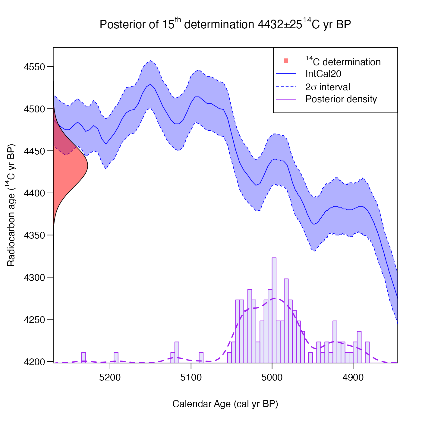
# Result for 15th determination
PlotCalendarAgeDensityIndividualSample(15, polya_urn_output)


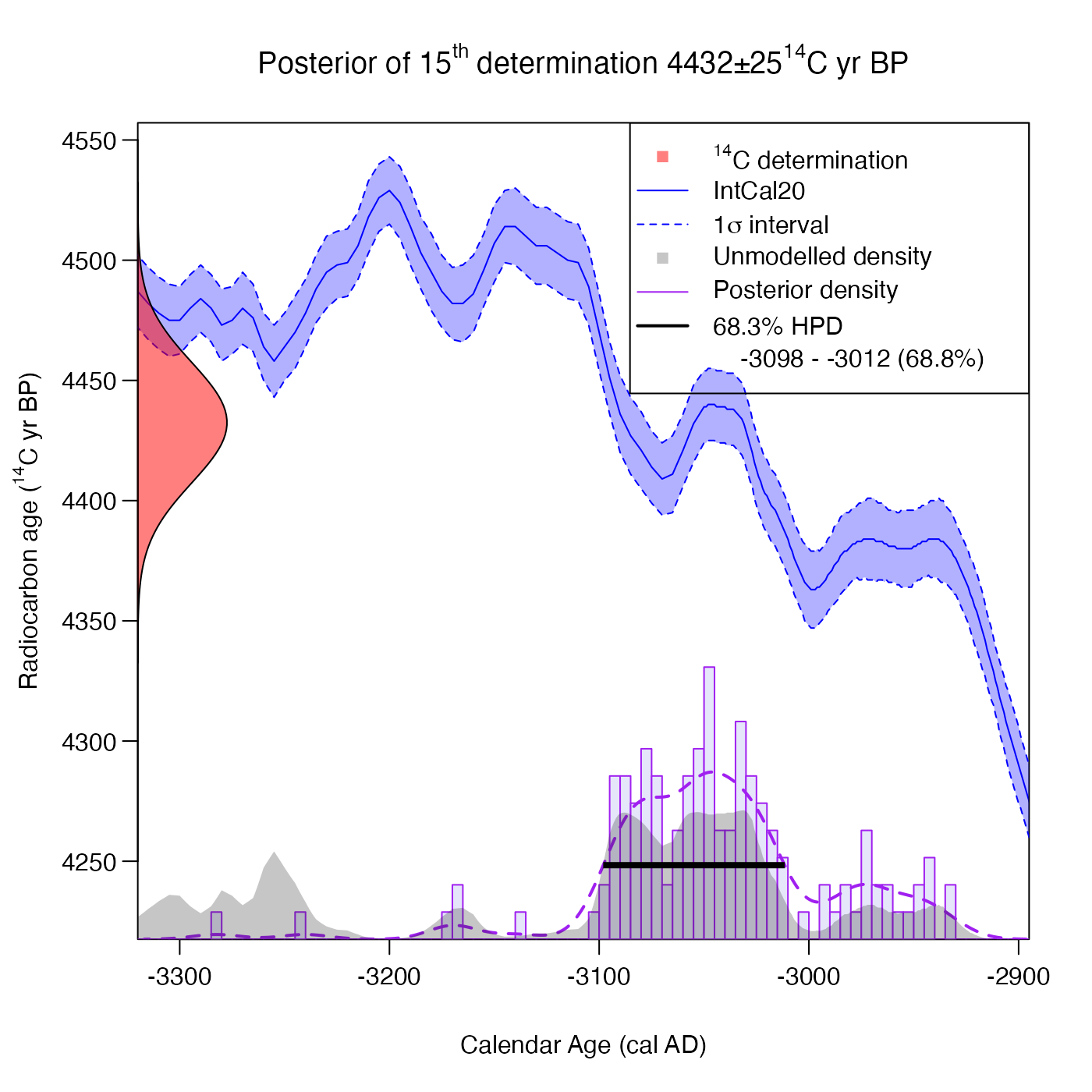
# Now change to show 1 sigma interval for HPD range and calibration curve
# and plot in yr AD
PlotCalendarAgeDensityIndividualSample(
    15,
    polya_urn_output,
    plot_cal_age_scale = "AD",
    interval_width = "1sigma",
    show_hpd_ranges = TRUE,
    show_unmodelled_density = TRUE)


# Plot and then assign the returned probability
posterior_dens <- PlotCalendarAgeDensityIndividualSample(15, polya_urn_output)

# Use this to find the mean posterior calendar age
weighted.mean(posterior_dens$calendar_age_BP, posterior_dens$probability)
#> [1] 4995.078

Usage

Arguments

Value

See also

Examples