Independent Single Sample Calibration

library(carbondate)

Introduction

This package is primarily concerned with the calibration, and summarisation, of multiple related ¹⁴C determinations. With such a set of samples, which are believed to arise from a common calendar distribution related to the culture/context under study, the calibration of those samples should be performed jointly. This will allow calendar age information to be shared between the samples during the calibration process leading to improved overall calibration accuracy. It also allows us to combine and summarise the calendar age information provided by the entire set.

However, our library also provides functions for calibrating a single ¹⁴C sample independently. This can be useful if one does only have a single ¹⁴C sample, or to provide comparison with the joint calibration approaches.

Independent Calibration of Single ¹⁴C Samples

To calibrate a single independent determination using the provided IntCal20 calibration curve (Reimer et al. 2020), run the following:

calibration_result <- CalibrateSingleDetermination(
  rc_determination = 1413, 
  rc_sigma = 25, 
  F14C_inputs = FALSE, 
  calibration_curve = intcal20,
  plot_output = TRUE)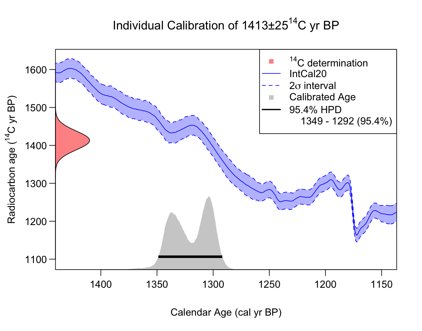

Implementing SH calibration

To change to using the Southern Hemisphere calibration curve SHCal20 (Hogg et al. 2020), we can modify the function arguments accordingly:

calibration_result <- CalibrateSingleDetermination(
  rc_determination = 1413, 
  rc_sigma = 25, 
  F14C_inputs = FALSE, 
  calibration_curve = shcal20,
  plot_output = TRUE)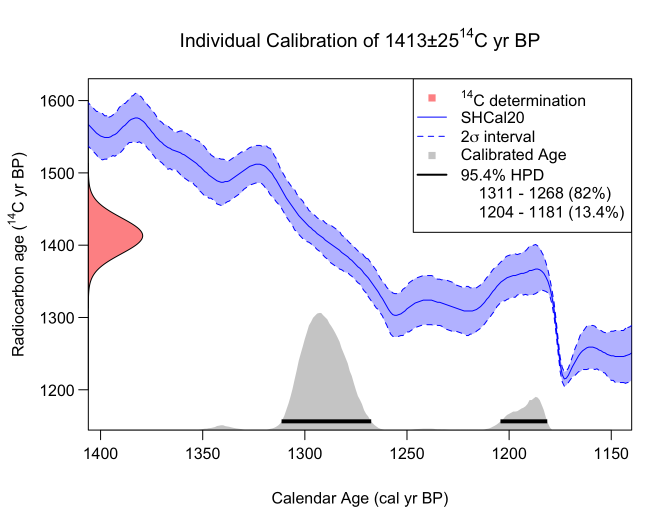

Note: This simulated SH calibration, of the same ¹⁴C determination as above, provides a slightly more recent estimate for the calendar due to the offset (the interhemispheric ¹⁴C gradient) between atmospheric ¹⁴C levels in the Southern and Northern Hemisphere.

Implementing Marine calibration

To change to using the Marine20 calibration curve (Heaton et al. 2020), we can alter the argument to select the inbuilt marine20 curve. To perform marine calibration, we must also provide an estimate for the localised $\Delta R$ (and its $1\sigma$ -uncertainty) by specifying delta_r and delta_r_sig:

calibration_result <- CalibrateSingleDetermination(
  rc_determination = 1413, 
  rc_sigma = 25, 
  F14C_inputs = FALSE, 
  calibration_curve = marine20,
  delta_r = 150,
  delta_r_sig = 50, 
  plot_output = TRUE)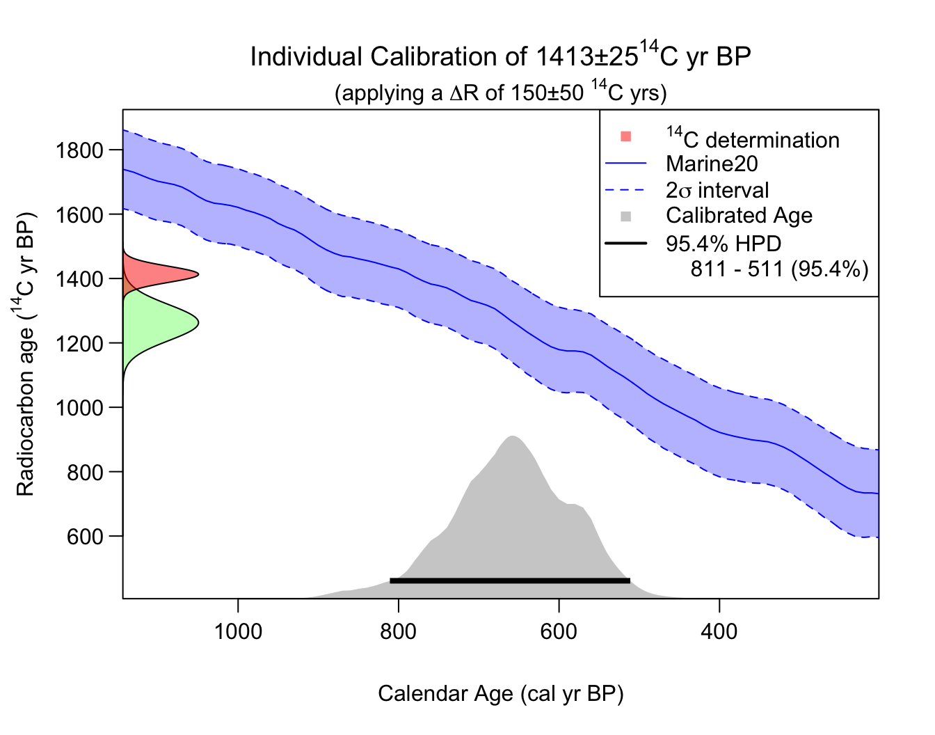

Here the radiocarbon age axis shows the analytical ¹⁴C determination in red, while the adjusted determination (after applying a $\Delta R = 150 \pm 50$ ¹⁴C yrs) is shown in green. Intuitively, we calibrate the green (adjusted) value against the Marine20 curve.

Note: One can also use the delta_r and delta_r_sig arguments to specify a general offset to a calibration curve (i.e., these arguments can also be used when using the IntCal and SHCal curves if the sample is thought to be offset).

Selecting the calendar age scale when plotting

All the calibration curves, and the outputs from our functions, are provided on the cal yr BP scale (where 0 cal yr BP = 1950 cal AD). However, for the plots, the user can alter the calendar age scale shown through the plot_cal_age_scale variable. The default is to plot the calendar ages on the cal yr BP scale (e.g., see above). To instead plot in cal AD, set plot_cal_age_scale = "AD"; while for cal BC set plot_cal_age_scale = "BC". For example,

calibration_result <- CalibrateSingleDetermination(
  rc_determination = 1413, 
  rc_sigma = 25, 
  F14C_inputs = FALSE, 
  calibration_curve = intcal20,
  plot_output = TRUE,
  plot_cal_age_scale = "AD")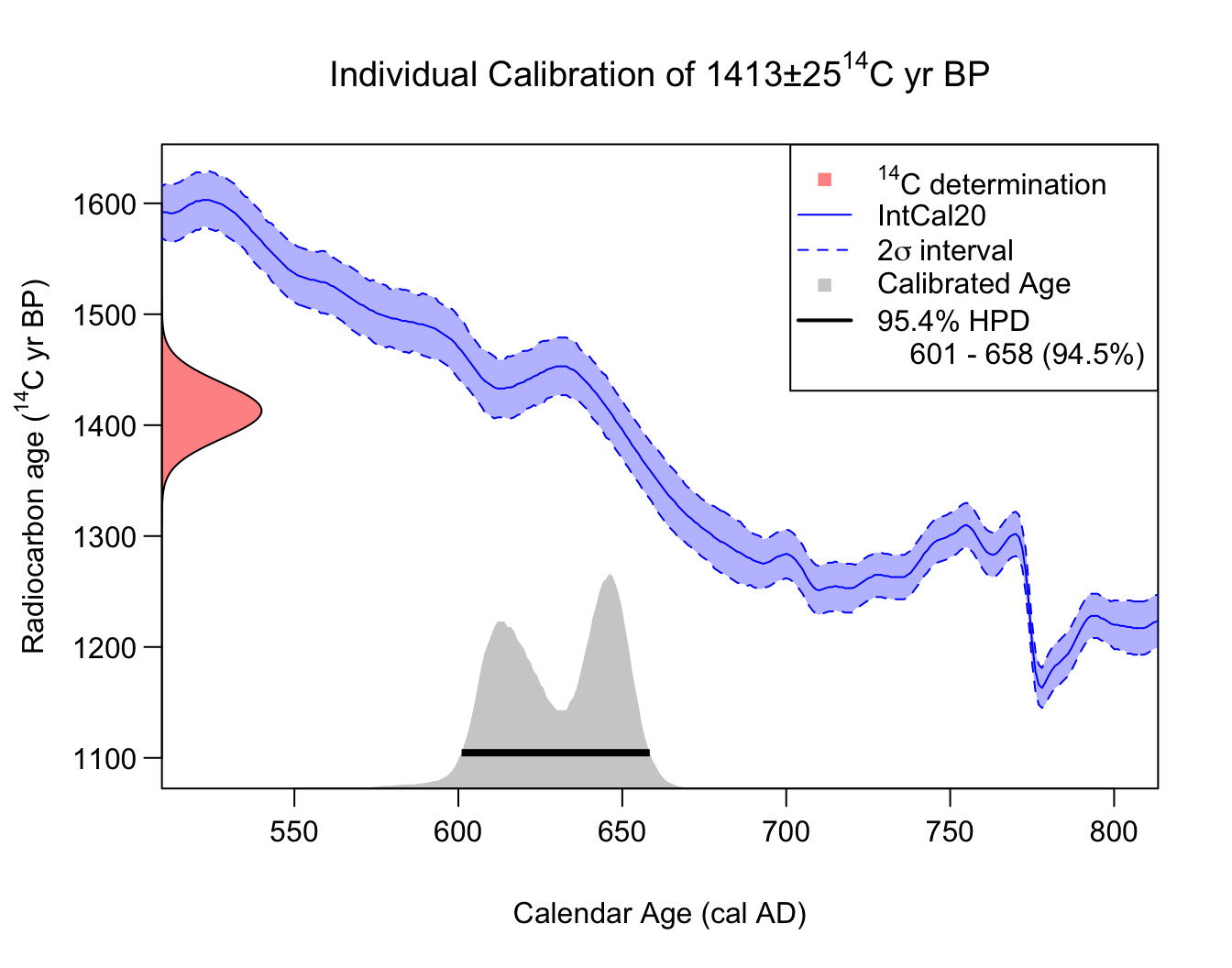

Annotating the plots with text, lines and shading

We have created three functions:

AddLinePlot() - adds lines (vertical or horizontal)
AddTextPlot() - adds text
AddShadingPlot() - adds shading

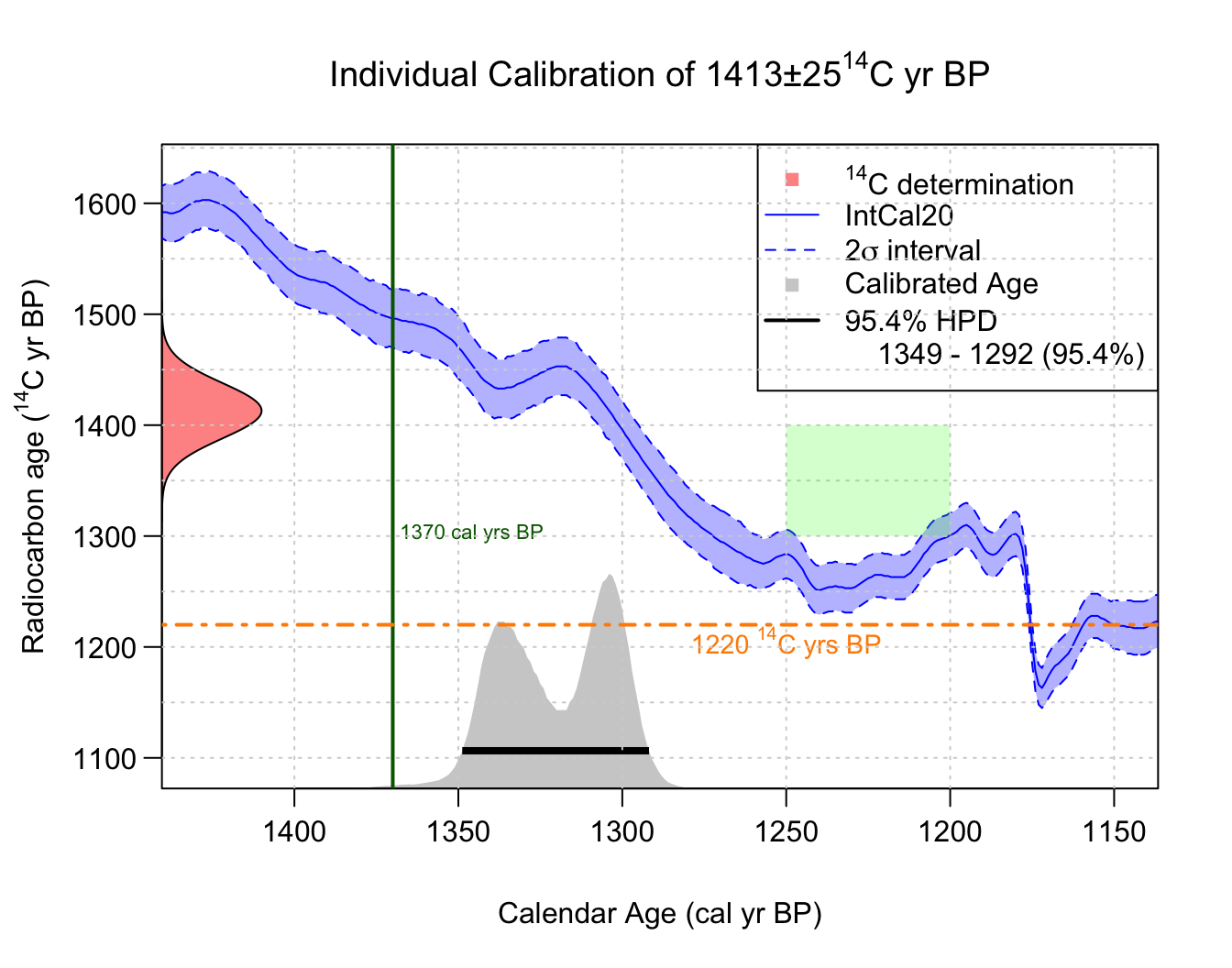
that allow you to annotate the posterior calendar age density plot. For example:

# Create initial plot
calibration_result_plot <- CalibrateSingleDetermination(
  rc_determination = 1413, 
  rc_sigma = 25, 
  F14C_inputs = FALSE, 
  calibration_curve = intcal20,
  plot_output = TRUE)

# Add solid vertical line at 1370 cal yr BP
AddLinePlot(calibration_result_plot,
  v = 1370,
  col = "darkgreen",
  lwd = 2,
  lty = 1)

AddTextPlot(calibration_result_plot,
  x = 1370, y = 1300,
  labels = expression(paste("1370 cal yrs BP")),
  cex = 0.7,
  pos = 4, # Places the text to the right
  offset = 0.2,
  col = "darkgreen")

# Add a dot-dashed horizontal line at 1220 14C yrs BP
AddLinePlot(calibration_result_plot,
  h = 1220,
  col = "darkorange",
  lwd = 2,
  lty = 4)
    
AddTextPlot(calibration_result_plot,
  x = 1250, y = 1220,
  labels = expression(paste("1220", " "^14, "C ", "yrs BP")),
  cex = 0.9,
  pos = 1, # Places text below 
  offset = 0.2,
  col = "darkorange")

# Add light gray grid lines to entire plot
AddLinePlot(calibration_result_plot,
  h = seq(1000, 1700, by = 50),
  v = seq(1100, 1600, by = 50),
  col = "lightgray",
  lty = 3)

# Add a shaded box to cover a period
AddShadingPlot(calibration_result_plot,
  x_start = 1250, x_end = 1200,
  y_start = 1300, y_end = 1400,
  col = "green", alpha = 0.2)

References

Heaton, Timothy J, Peter Köhler, Martin Butzin, et al. 2020. “Marine20 — The Marine Radiocarbon Age Calibration Curve (0–55,000 cal BP).” Radiocarbon 62 (4): 779–820. https://doi.org/10.1017/RDC.2020.68.

Hogg, Alan G, Timothy J Heaton, Quan Hua, et al. 2020. “SHCal20 Southern Hemisphere Calibration, 0–55,000 Years cal BP.” Radiocarbon 62 (4): 759–78. https://doi.org/10.1017/RDC.2020.59.

Reimer, Paula J, William E N Austin, Edouard Bard, et al. 2020. “The IntCal20 Northern Hemisphere Radiocarbon Age Calibration Curve (0–55 cal kBP).” Radiocarbon 62 (4): 725–57. https://doi.org/10.1017/rdc.2020.41.