Summed Probability Distributions
Currently, the most commonly-used approach to summarise calendar age information from multiple 14C determinations is to calculate the summed probability distribution (SPD). However, SPDs provide neither reliable nor statistically valid estimation of the summarised calendar age information. It is our view that they should not be used in any dates-as-data approach to provide a population proxy. For complete details, with comprehensive illustrative examples, on why SPDs should not be used for summarisation and how they can provide highly misleading inference, see (Heaton et al. 2025)).
The Problems with using SPDs
When creating an SPD, the posterior calendar age density of each object is first calculated independently from the others. These individual densities are then summed/averaged to give an SPD estimate. The independence assumed in the initial calibration of each sample, is fundamentally contradictory to the subsequent summarisation and results in a calendar age summary that is both unreliable and inconsistent.
Additionally, the SPD approach fundamentally does not model the samples in the calendar age domain. Consequently, it is also not able to deal with inversions in the calibration curve where there are multiple disjoint calendar periods which are consistent with the observed determinations; or with plateau periods.
The SPD function is ONLY provided here as a
comparison with the other routines. To calculate the SPD for a set of
radiocarbon determinations (here we use the example dataset
armit (Armit et al. 2014))
see the example below, where we also plot the results.
spd <- FindSummedProbabilityDistribution(
  calendar_age_range_BP = c(1000, 4500),
  rc_determinations = armit$c14_age,
  rc_sigmas = armit$c14_sig,
  F14C_inputs = FALSE,
  calibration_curve = intcal20,
  plot_output = TRUE)
Note: The functions we provide to plot the rigorous calendar age summary provided by our Bayesian non-parametric DPMM alternative to SPDs can also optionally plot the SPD - see the vignette Non-parametric Calendar Age Summarisation for details.
Illustration of why not to use SPDs
Fitting to a mixture of two normal distributions
The two_normals dataset contains 50 simulated
14C determinations. These were created by first drawing a set
of 50 calendar ages from a mixture of two normal calendar age densities
- one centred at 3500 cal yr BP (with a
1
standard deviation of 200 cal yrs); and another (more concentrated)
centred at 5000 cal yr BP (with a
1
standard deviation of 100 cal yrs). Having simulated these calendar
ages, a corresponding 14C determination for each sample were
created using the IntCal20 curve (Reimer et al.
2020).
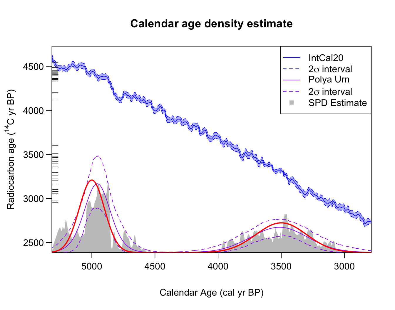
When we summarise the calendar age information provided by the 50 simulated 14C determinations, we would aim to reconstruct the underying mixture of two normals that were used to generate the data. However, when we calculate the SPD we obtain:
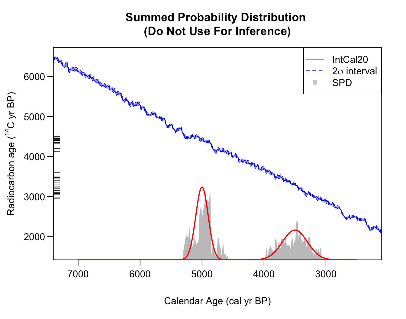
Here we have manually overlain the true (in this case, known) shared calendar age density in red. As we can see, the SPD captures does capture some broad features of that underlying calendar age distribution but does not reconstruct the truth well, and is hard to interpret. In particular, the SPD is highly variable, showing multiple peaks, due to the wiggliness of the calibration curve. The SPD peak shown around 5300 cal yr BP is entirely spurious, yet almost of the same magnitude as its peak around 3500 cal yr BP (which is a part of the genuine density).