Plot Posterior Mean Rate of Sample Occurrence for Poisson Process Model
Source:R/PlotPosteriorMeanRate.R
PlotPosteriorMeanRate.RdGiven output from the Poisson process fitting function PPcalibrate calculate and plot the posterior mean rate of sample occurrence (i.e., the underlying Poisson process rate \(\lambda(t)\)) together with specified probability intervals, on a given calendar age grid (provided in cal yr BP).
Will show the original set of radiocarbon determinations (those you are modelling/summarising), the chosen calibration curve, and the estimated posterior rate of occurrence \(\lambda(t)\) on the same plot. Can also optionally show the posterior mean of each individual sample's calendar age estimate.
An option is also provided to calculate the posterior mean rate conditional upon the number of internal changepoints within the period under study (if this is specified as an input to the function).
Note: If all you are interested in is the value of the posterior mean rate on a grid, without an accompanying plot, you can use FindPosteriorMeanRate instead.
For more information read the vignette: vignette("Poisson-process-modelling", package = "carbondate")
Usage
PlotPosteriorMeanRate(
  output_data,
  n_posterior_samples = 5000,
  n_changes = NULL,
  calibration_curve = NULL,
  plot_14C_age = TRUE,
  plot_cal_age_scale = "BP",
  show_individual_means = TRUE,
  show_confidence_intervals = TRUE,
  interval_width = "2sigma",
  bespoke_probability = NA,
  denscale = 3,
  resolution = 1,
  n_burn = NA,
  n_end = NA,
  plot_pretty = TRUE,
  plot_lwd = 2
)
Arguments
- output_data
The return value from the updating function PPcalibrate. Optionally, the output data can have an extra list item named
labelwhich is used to set the label on the plot legend.- n_posterior_samples
Number of samples it will draw, after having removed
n_burn, from the (thinned) MCMC realisations stored inoutput_datato estimate the rate \(\lambda(t)\). These samples may be repeats if the number of, post burn-in, realisations is less thann_posterior_samples. If not given, 5000 is used.- n_changes
(Optional) If wish to condition calculation of the posterior mean on the number of internal changepoints. In this function, if specified,
n_changesmust be a single integer.- calibration_curve
This is usually not required since the name of the calibration curve variable is saved in the output data. However, if the variable with this name is no longer in your environment then you should pass the calibration curve here. If provided, this should be a dataframe which should contain at least 3 columns entitled
calendar_age,c14_ageandc14_sig. This format matches intcal20.- plot_14C_age
Whether to use the radiocarbon age (\({}^{14}\)C yr BP) as the units of the y-axis in the plot. Defaults to
TRUE. IfFALSEuses F\({}^{14}\)C concentration instead.- plot_cal_age_scale
(Optional) The calendar scale to use for the x-axis. Allowed values are "BP", "AD" and "BC". The default is "BP" corresponding to plotting in cal yr BP.
- show_individual_means
(Optional) Whether to calculate and show the mean posterior calendar age estimated for each individual \({}^{14}\)C sample on the plot as a rug on the x-axis. Default is
TRUE.- show_confidence_intervals
Whether to show the pointwise confidence intervals (at chosen probability level) on the plot. Default is
TRUE.- interval_width
The confidence intervals to show for both the calibration curve and the predictive density. Choose from one of
"1sigma"(68.3%),"2sigma"(95.4%) and"bespoke". Default is"2sigma".- bespoke_probability
The probability to use for the confidence interval if
"bespoke"is chosen above. E.g., if 0.95 is chosen, then the 95% confidence interval is calculated. Ignored if"bespoke"is not chosen.- denscale
(Optional) Whether to scale the vertical range of the Poisson process mean rate plot relative to the calibration curve plot. Default is 3 which means that the maximum of the mean rate will be at 1/3 of the height of the plot.
- resolution
The distance between calendar ages at which to calculate the value of the rate \(\lambda(t)\). These ages will be created on a regular grid that automatically covers the calendar period specified in
output_data. Default is 1.- n_burn
The number of MCMC iterations that should be discarded as burn-in (i.e., considered to be occurring before the MCMC has converged). This relates to the number of iterations (
n_iter) when running the original update functions (not the thinnedoutput_data). Any MCMC iterations before this are not used in the calculations. If not given, the first half of the MCMC chain is discarded. Note: The maximum value that the function will allow isn_iter - 100 * n_thin(wheren_iterandn_thinare the arguments that were given to PPcalibrate) which would leave only 100 of the (thinned) values inoutput_data.- n_end
The last iteration in the original MCMC chain to use in the calculations. Assumed to be the total number of iterations performed, i.e.
n_iter, if not given.- plot_pretty
logical, defaulting to
TRUE. If setTRUEthen will select pretty plotting margins (that create sufficient space for axis titles and rotates y-axis labels). IfFALSEwill implement current user values.- plot_lwd
The line width to use when plotting the posterior mean (and confidence intervals). Default is 2 (to add emphasis).
Value
A list, each item containing a data frame of the calendar_age_BP, the rate_mean
and the confidence intervals for the rate - rate_ci_lower and rate_ci_upper.
Examples
# NOTE: All these examples are shown with a small n_iter and n_posterior_samples
# to speed up execution.
# Try n_iter and n_posterior_samples as the function defaults.
pp_output <- PPcalibrate(
pp_uniform_phase$c14_age,
pp_uniform_phase$c14_sig,
intcal20,
n_iter = 1000,
show_progress = FALSE)
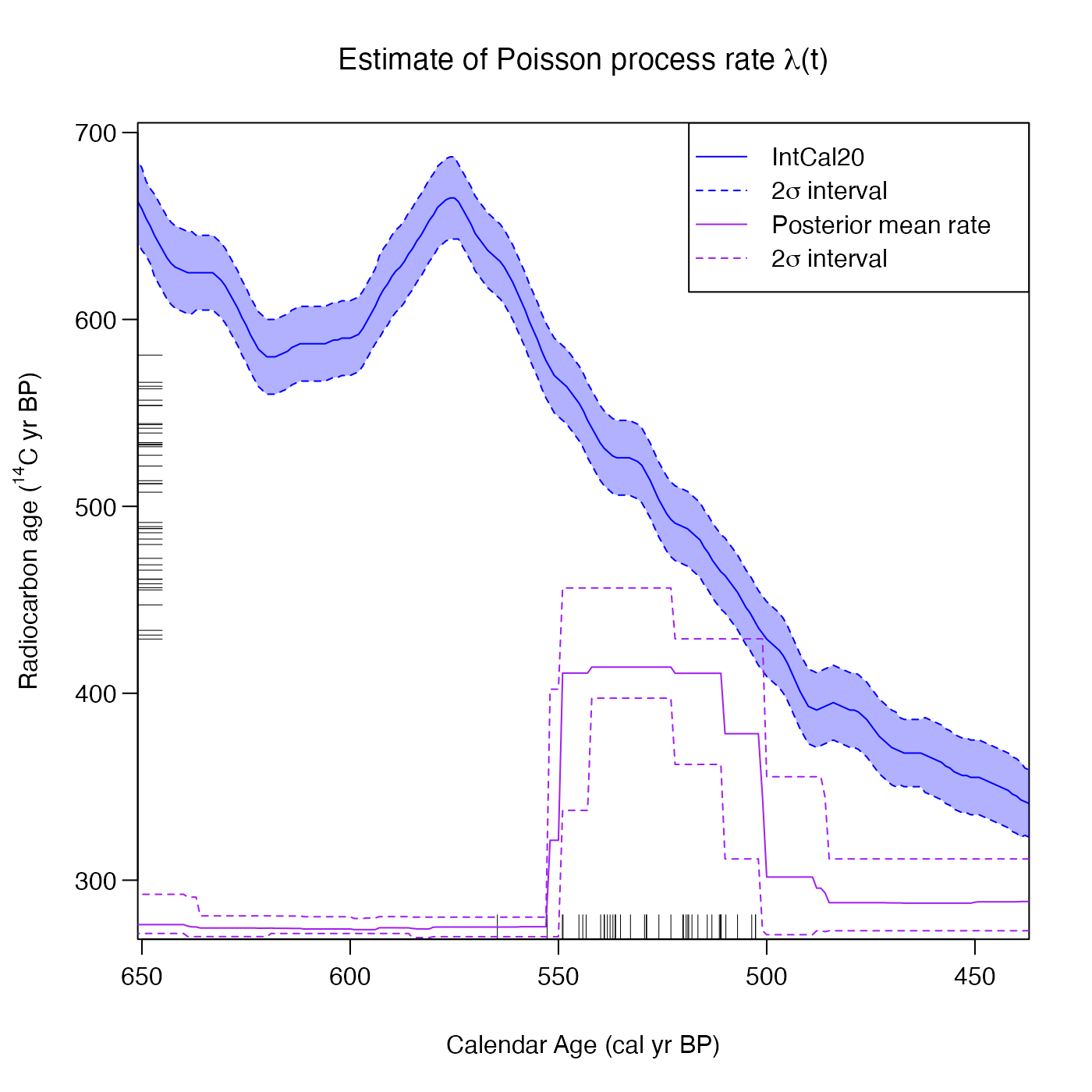
# Default plot with 2 sigma interval
PlotPosteriorMeanRate(pp_output, n_posterior_samples = 100)
 # Decrease the line width of the posterior mean
PlotPosteriorMeanRate(pp_output, n_posterior_samples = 100, plot_lwd = 1)
# Decrease the line width of the posterior mean
PlotPosteriorMeanRate(pp_output, n_posterior_samples = 100, plot_lwd = 1)
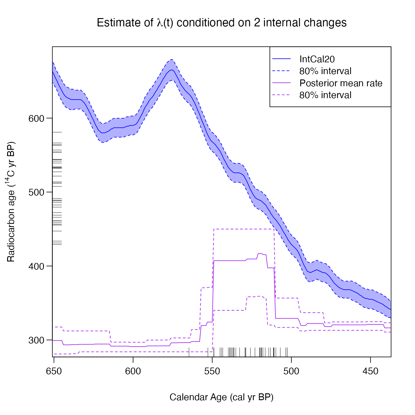
 # Specify an 80% confidence interval
PlotPosteriorMeanRate(
pp_output,
interval_width = "bespoke",
bespoke_probability = 0.8,
n_posterior_samples = 100)
# Specify an 80% confidence interval
PlotPosteriorMeanRate(
pp_output,
interval_width = "bespoke",
bespoke_probability = 0.8,
n_posterior_samples = 100)
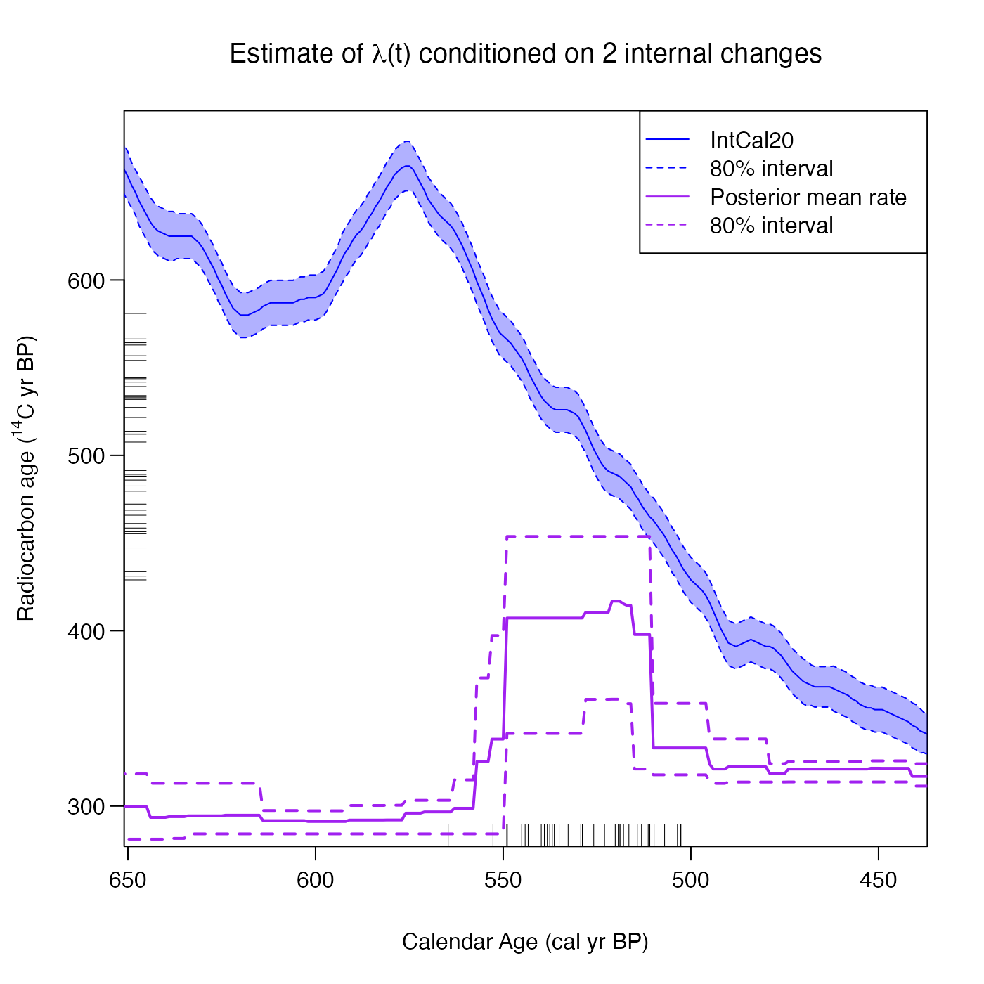
 # Plot the posterior rate conditional on 2 internal changes
PlotPosteriorMeanRate(
pp_output,
n_changes = 2,
interval_width = "bespoke",
bespoke_probability = 0.8,
n_posterior_samples = 100)
#> Warning: Only 16 posterior samples with 2 internal changes, so results may not be robust. Try running the original MCMC for longer, or increasing n_posterior_samples
# Plot the posterior rate conditional on 2 internal changes
PlotPosteriorMeanRate(
pp_output,
n_changes = 2,
interval_width = "bespoke",
bespoke_probability = 0.8,
n_posterior_samples = 100)
#> Warning: Only 16 posterior samples with 2 internal changes, so results may not be robust. Try running the original MCMC for longer, or increasing n_posterior_samples