Add Straight Lines to Various Summary Plots

Having plotted the output of the various modelling approaches, add one or more straight lines to the current plot. It is based on the base abline function

This function/annotation can be applied after having called any of PlotPosteriorMeanRate, PlotPosteriorChangePoints, CalibrateSingleDetermination, PlotPredictiveCalendarAgeDensity, PlotCalendarAgeDensityIndividualSample, or PlotRateIndividualRealisation.

Usage

AddLinePlot(
  output_plot,
  a = NULL,
  b = NULL,
  h = NULL,
  v = NULL,
  reg = NULL,
  coef = NULL,
  ...
)

Arguments

output_plot

The plot onto which you wish to add text

a, b

the intercept and slope, single values.

h

the y-value(s) for horizontal line(s).

v

the x-value(s) for vertical line(s).

reg

An object with a coef method

coef

a vector of length two giving the intercept and slope.

...

graphical parameters such as col, lty and lwd (possibly as vectors: see ‘Details’) and xpd and the line characteristics lend, ljoin and lmitre.

Value

None

Examples

# NOTE: This example is shown with a small n_iter and n_posterior_samples
# to speed up execution.
# Try n_iter and n_posterior_samples as the function defaults.

pp_output <- PPcalibrate(
    pp_uniform_phase$c14_age,
    pp_uniform_phase$c14_sig,
    intcal20,
    n_iter = 1000,
    show_progress = FALSE)

# Default plot with 2 sigma interval
posterior_mean_plot <- PlotPosteriorMeanRate(
    pp_output,
    n_posterior_samples = 100)

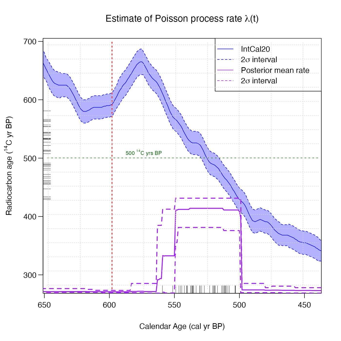
# Add vertical thick red dashed line to plot
AddLinePlot(
     posterior_mean_plot,
     v = 600,
     col = "red",
     lwd = 2,
     lty = 3)

# Add narrow horizontal green dashed line
AddLinePlot(
     posterior_mean_plot,
     h = 500,
     col = "darkgreen",
     lwd = 1,
     lty = 2)

# Add text to annotate line
AddTextPlot(posterior_mean_plot,
    x = 575, y = 500,
    labels = expression(paste("500", " "^14, "C ", "yrs BP")),
    cex = 0.7,
    pos = 3,
    offset = 0.2,
    col = "darkgreen")

# Add light gray grid lines
AddLinePlot(posterior_mean_plot,
     posterior_mean_plot,
     h = seq(250, 700, by = 25),
     v = seq(400, 650, by = 25),
     col = "lightgray",
     lty = 3)