Find the summed probability distribution (SPD) for a set of radiocarbon observations

Takes a set of radiocarbon determinations and uncertainties, independently calibrates each one, and then averages the resultant calendar age estimates to give the SPD estimate.

Important: This function should not be used for inference as SPDs are not statistically rigorous. Instead use either of:

the Bayesian non-parametric summarisation approaches PolyaUrnBivarDirichlet or WalkerBivarDirichlet;
or the Poisson process rate approach PPcalibrate

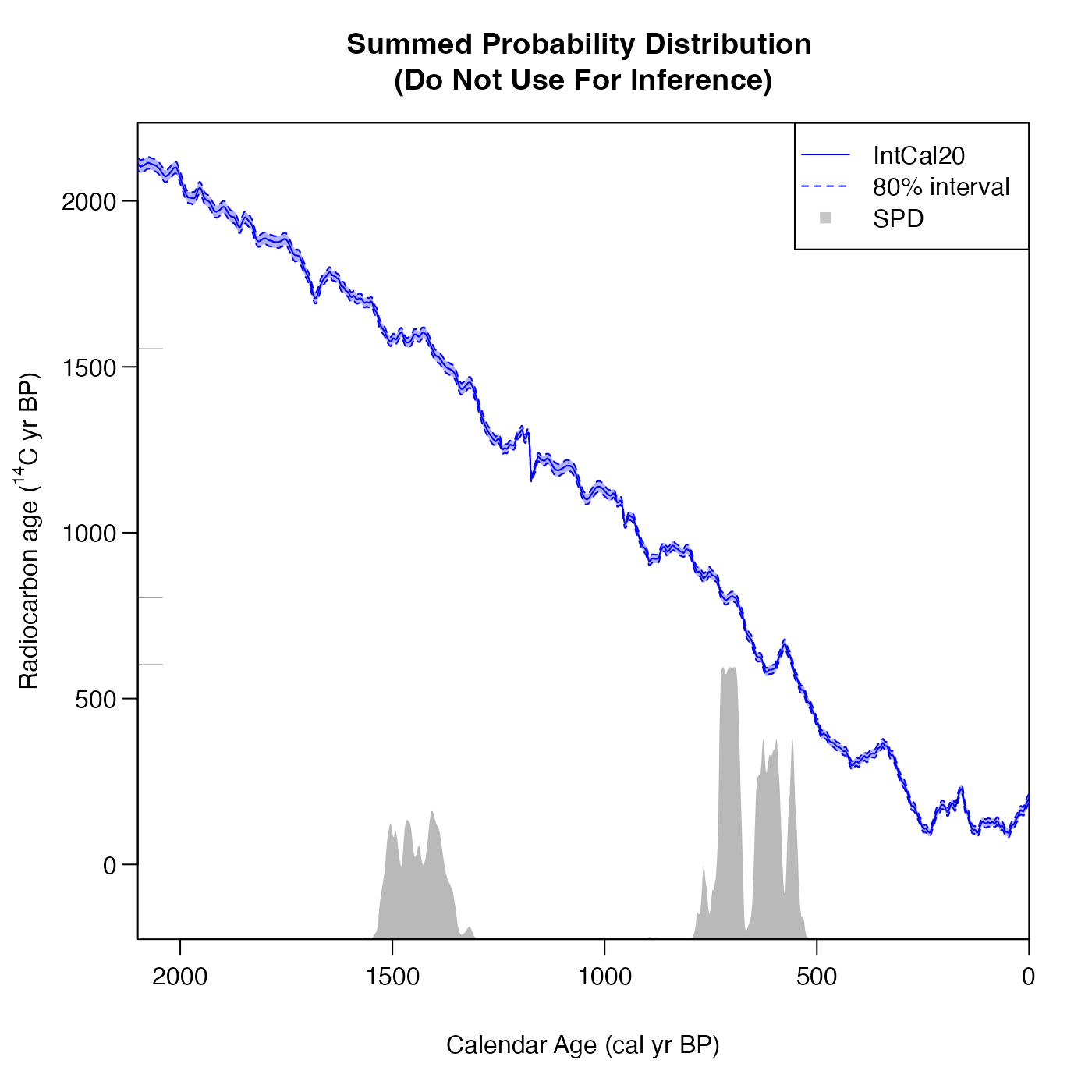
The SPD function provided here is only intended for comparison. We provide a inbuilt plotting option to show the SPD alongside the determinations and the calibration curve.

Usage

FindSummedProbabilityDistribution(
  calendar_age_range_BP,
  rc_determinations,
  rc_sigmas,
  calibration_curve,
  F14C_inputs = FALSE,
  resolution = 1,
  plot_output = FALSE,
  plot_cal_age_scale = "BP",
  interval_width = "2sigma",
  bespoke_probability = NA,
  denscale = 3,
  plot_pretty = TRUE
)

Arguments

calendar_age_range_BP: A vector of length 2 with the start and end calendar age BP to calculate the SPD over. These two values must be in order with start value less than end value, e.g., (600, 1700) cal yr BP. The code will extend this range (by 400 cal yrs each side) for conservativeness
rc_determinations: A vector of observed radiocarbon determinations. Can be provided either as \({}^{14}\)C ages (in \({}^{14}\)C yr BP) or as F\({}^{14}\)C concentrations.
rc_sigmas: A vector of the (1-sigma) measurement uncertainties for the radiocarbon determinations. Must be the same length as rc_determinations and given in the same units.
calibration_curve: A dataframe which must contain one column calendar_age_BP, and also columns c14_age and c14_sig or f14c and f14c_sig (or both sets). This format matches the curves supplied with this package, e.g., intcal20, intcal13, which contain all 5 columns.
F14C_inputs: TRUE if the provided rc_determinations are F\({}^{14}\)C concentrations and FALSE if they are radiocarbon ages. Defaults to FALSE.
resolution: The distance between the calendar ages at which to calculate the calendar age probability. Default is 1.
plot_output: TRUE if you wish to plot the determinations, the calibration curve, and the SPD on the same plot. Defaults to FALSE
plot_cal_age_scale: Only for usage when plot_output = TRUE. The calendar scale to use for the x-axis. Allowed values are "BP", "AD" and "BC". The default is "BP", corresponding to plotting in cal yr BP.
interval_width: Only for usage when plot_output = TRUE. The confidence intervals to show for the calibration curve. Choose from one of "1sigma" (68.3%), "2sigma" (95.4%) and "bespoke". Default is "2sigma".
bespoke_probability: The probability to use for the confidence interval if "bespoke" is chosen above. E.g. if 0.95 is chosen, then the 95% confidence interval is calculated. Ignored if "bespoke" is not chosen.
denscale: Whether to scale the vertical range of the calendar age density plot relative to the calibration curve plot (optional). Default is 3 which means that the maximum SPD will be at 1/3 of the height of the plot.
plot_pretty: logical, defaulting to TRUE. If set TRUE then will select pretty plotting margins (that create sufficient space for axis titles and rotates y-axis labels). If FALSE will implement current user values.

Value

A data frame with one column calendar_age_BP containing the calendar ages, and the other column probability containing the probability at that calendar age

Examples

# An example using 14C age BP and the IntCal 20 curve
SPD <- FindSummedProbabilityDistribution(
   calendar_age_range_BP=c(400, 1700),
   rc_determinations=c(602, 805, 1554),
   rc_sigmas=c(35, 34, 45),
   calibration_curve=intcal20)
plot(SPD, type = "l",
   xlim = rev(range(SPD$calendar_age_BP)),
   xlab = "Calendar Age (cal yr BP)")


# Using the inbuilt plotting features
SPD <- FindSummedProbabilityDistribution(
   calendar_age_range_BP=c(400, 1700),
   rc_determinations=c(602, 805, 1554),
   rc_sigmas=c(35, 34, 45),
   calibration_curve=intcal20,
   plot_output = TRUE,
   interval_width = "bespoke",
   bespoke_probability = 0.8)


# An different example using F14C concentrations and the IntCal 13 curve
SPD <- FindSummedProbabilityDistribution(
   calendar_age_range_BP=c(400, 2100),
   rc_determinations=c(0.8, 0.85, 0.9),
   rc_sigmas=c(0.01, 0.015, 0.012),
   F14C_inputs=TRUE,
   calibration_curve=intcal13)
plot(SPD, type = "l",
   xlim = rev(range(SPD$calendar_age_BP)),
   xlab = "Calendar Age (cal yr BP)")

Usage

Arguments

Value

See also

Examples