Plot Number of Changepoints in Rate of Sample Occurrence for Poisson Process Model

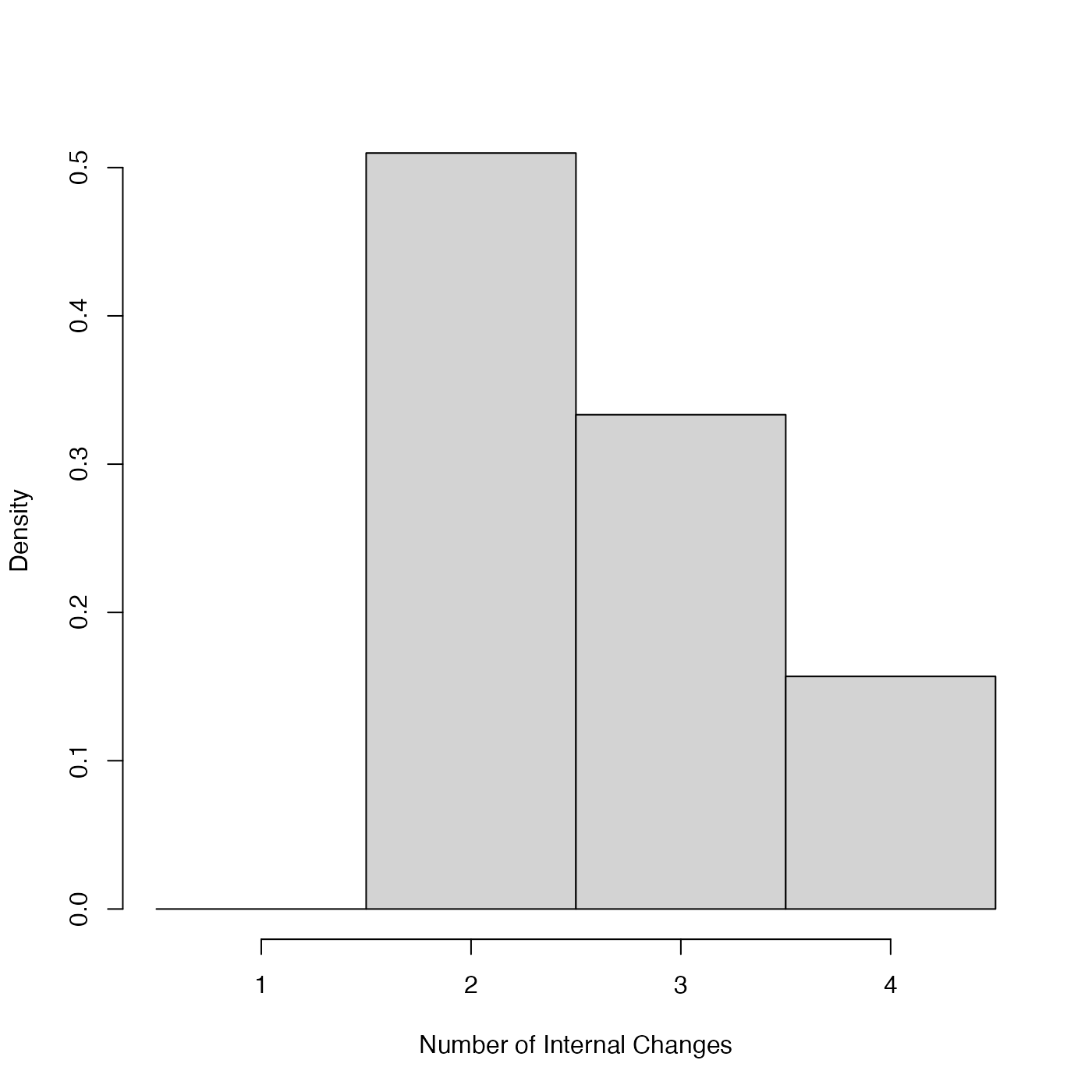
Given output from the Poisson process fitting function PPcalibrate, plot the posterior distribution for the number of internal changepoints in the underlying rate of sample occurrence (i.e., in \(\lambda(t)\)) over the period under study.

For more information read the vignette:
vignette("Poisson-process-modelling", package = "carbondate")

Usage

PlotNumberOfInternalChanges(output_data, n_burn = NA, n_end = NA)

Arguments

output_data

The return value from the updating function PPcalibrate. Optionally, the output data can have an extra list item named label which is used to set the label on the plot legend.

n_burn

The number of MCMC iterations that should be discarded as burn-in (i.e., considered to be occurring before the MCMC has converged). This relates to the number of iterations (n_iter) when running the original update functions (not the thinned output_data). Any MCMC iterations before this are not used in the calculations. If not given, the first half of the MCMC chain is discarded. Note: The maximum value that the function will allow is n_iter - 100 * n_thin (where n_iter and n_thin are the arguments that were given to PPcalibrate) which would leave only 100 of the (thinned) values in output_data.

n_end

The last iteration in the original MCMC chain to use in the calculations. Assumed to be the total number of iterations performed, i.e. n_iter, if not given.

Value

None

Examples

# NOTE: This example is shown with a small n_iter to speed up execution.
# Try n_iter and n_posterior_samples as the function defaults.

pp_output <- PPcalibrate(
    pp_uniform_phase$c14_age,
    pp_uniform_phase$c14_sig,
    intcal20,
    n_iter = 1000,
    show_progress = FALSE)

PlotNumberOfInternalChanges(pp_output)